3: IceNet Data and Forecast Products#
Context#
Purpose#
The IceNet library provides the ability to download, process, train and predict from end to end via a set of command-line interfaces (CLI).
Using this notebook one can understand the various data sources, intermediaries and products that arise from both the CLI demonstrator notebook and Pipeline demonstrate notebook activities.
Modelling approach#
This modelling approach allows users to immediately utilise the library for producing sea ice concentraion forecasts.
Highlights#
The key features of an end to end run are:
Setup: this was concerned with setting up the conda environment, which remains the same
1. Download: we explore the source data downloaded under the
/data/folder, reusable across multiple environments2. Process: we explore the preprocessing outputs in the
/processed/folder, which can be fed to models directly or further processed into IceNet datasets3. Train: we explore the outputs from the training process and ensemble runs, stored within
/results/networks/4. Predict: we explore the output from the prediction process and ensemble runs, stored within
/results/predict/
This follows the same structure as the CLI demonstration notebook so that it’s easy to follow step-by-step…
Contributions#
Notebook#
James Byrne (author)
Bryn Noel Ubald (co-author)
Please raise issues in this repository to suggest updates to this notebook!
Contact me at jambyr <at> bas.ac.uk for anything else…
Modelling codebase#
James Byrne (code author), Bryn Noel Ubald (code author), Tom Andersson (science author)
Modelling publications#
Andersson, T.R., Hosking, J.S., Pérez-Ortiz, M. et al. Seasonal Arctic sea ice forecasting with probabilistic deep learning. Nat Commun 12, 5124 (2021). https://doi.org/10.1038/s41467-021-25257-4
Involved organisations#
The Alan Turing Institute and British Antarctic Survey
Setup#
For the purposes of python analysis we use and provide the following header libraries which are heavily utilised within the IceNet project and the pipeline.
import glob, json, os
import datetime as dt
import pandas as pd, xarray as xr, matplotlib.pyplot as plt
from IPython.display import HTML
%matplotlib inline
1. Download#
Downloading data using the icenet_data commands produces a dataset specific input data storage directory called /data whose source data can be reused across normalisation (icenet_process*) and dataset production (icenet_dataset*) runs.
os.listdir("data")
['masks', 'era5', 'osisaf']
The structure of these directories (aside from masks) have consistent layouts:
glob.glob("data/**/2020.nc", recursive=True)
['data/era5/north/psl/2020.nc',
'data/era5/north/ta500/2020.nc',
'data/era5/north/tas/2020.nc',
'data/era5/north/tos/2020.nc',
'data/era5/north/uas/2020.nc',
'data/era5/north/vas/2020.nc',
'data/era5/north/zg250/2020.nc',
'data/era5/north/zg500/2020.nc',
'data/era5/south/psl/2020.nc',
'data/era5/south/ta500/2020.nc',
'data/era5/south/tas/2020.nc',
'data/era5/south/tos/2020.nc',
'data/era5/south/uas/2020.nc',
'data/era5/south/vas/2020.nc',
'data/era5/south/zg250/2020.nc',
'data/era5/south/zg500/2020.nc',
'data/osisaf/south/siconca/2020.nc']
With masks being the only caveat. However, masks can be interacted with purely through the Masks class from icenet.data.sic.mask.
glob.glob("data/masks/**/*.*", recursive=True)
['data/masks/south/masks/masks.params',
'data/masks/south/masks/active_grid_cell_mask_01.npy',
'data/masks/south/masks/land_mask.npy',
'data/masks/south/masks/active_grid_cell_mask_02.npy',
'data/masks/south/masks/active_grid_cell_mask_03.npy',
'data/masks/south/masks/active_grid_cell_mask_04.npy',
'data/masks/south/masks/active_grid_cell_mask_05.npy',
'data/masks/south/masks/active_grid_cell_mask_06.npy',
'data/masks/south/masks/active_grid_cell_mask_07.npy',
'data/masks/south/masks/active_grid_cell_mask_08.npy',
'data/masks/south/masks/active_grid_cell_mask_09.npy',
'data/masks/south/masks/active_grid_cell_mask_10.npy',
'data/masks/south/masks/active_grid_cell_mask_11.npy',
'data/masks/south/masks/active_grid_cell_mask_12.npy',
'data/masks/south/siconca/2000/01/ice_conc_sh_ease2-250_cdr-v2p0_200001021200.nc',
'data/masks/south/siconca/2000/02/ice_conc_sh_ease2-250_cdr-v2p0_200002021200.nc',
'data/masks/south/siconca/2000/03/ice_conc_sh_ease2-250_cdr-v2p0_200003021200.nc',
'data/masks/south/siconca/2000/04/ice_conc_sh_ease2-250_cdr-v2p0_200004021200.nc',
'data/masks/south/siconca/2000/05/ice_conc_sh_ease2-250_cdr-v2p0_200005021200.nc',
'data/masks/south/siconca/2000/06/ice_conc_sh_ease2-250_cdr-v2p0_200006021200.nc',
'data/masks/south/siconca/2000/07/ice_conc_sh_ease2-250_cdr-v2p0_200007021200.nc',
'data/masks/south/siconca/2000/08/ice_conc_sh_ease2-250_cdr-v2p0_200008021200.nc',
'data/masks/south/siconca/2000/09/ice_conc_sh_ease2-250_cdr-v2p0_200009021200.nc',
'data/masks/south/siconca/2000/10/ice_conc_sh_ease2-250_cdr-v2p0_200010021200.nc',
'data/masks/south/siconca/2000/11/ice_conc_sh_ease2-250_cdr-v2p0_200011021200.nc',
'data/masks/south/siconca/2000/12/ice_conc_sh_ease2-250_cdr-v2p0_200012021200.nc']
Note that the siconca variable files are source files for generating the masks that are not actually used after initial mask creation.
Producing data source videos#
One of the easiest ways to inspect source data is to use the icenet_video_data command, which will output to /plot/ in the run directory video(s) corresponding to the selected dataset, hemisphere, variable and year, or all of these items if run with:
!icenet_video_data --years 2020 era5,osisaf
[18-02-25 17:22:14 :INFO ] - Looking into data
[18-02-25 17:22:14 :INFO ] - Looking at data
[18-02-25 17:22:14 :INFO ] - Looking at data/era5
[18-02-25 17:22:14 :INFO ] - Looking at data/era5/north
[18-02-25 17:22:14 :INFO ] - Looking at data/era5/north/psl
[18-02-25 17:22:14 :INFO ] - Looking at data/era5/north/siconca
[18-02-25 17:22:14 :INFO ] - Looking at data/era5/north/ta500
[18-02-25 17:22:14 :INFO ] - Looking at data/era5/north/tas
[18-02-25 17:22:14 :INFO ] - Looking at data/era5/north/tos
[18-02-25 17:22:14 :INFO ] - Looking at data/era5/north/uas
[18-02-25 17:22:14 :INFO ] - Looking at data/era5/north/vas
[18-02-25 17:22:14 :INFO ] - Looking at data/era5/north/zg250
[18-02-25 17:22:14 :INFO ] - Looking at data/era5/north/zg500
[18-02-25 17:22:14 :INFO ] - Looking at data/era5/south
[18-02-25 17:22:14 :INFO ] - Looking at data/era5/south/psl
[18-02-25 17:22:14 :INFO ] - Looking at data/era5/south/siconca
[18-02-25 17:22:14 :INFO ] - Looking at data/era5/south/ta500
[18-02-25 17:22:14 :INFO ] - Looking at data/era5/south/tas
[18-02-25 17:22:14 :INFO ] - Looking at data/era5/south/tos
[18-02-25 17:22:14 :INFO ] - Looking at data/era5/south/uas
[18-02-25 17:22:14 :INFO ] - Looking at data/era5/south/vas
[18-02-25 17:22:14 :INFO ] - Looking at data/era5/south/zg250
[18-02-25 17:22:14 :INFO ] - Looking at data/era5/south/zg500
[18-02-25 17:22:14 :INFO ] - Looking at data/osisaf
[18-02-25 17:22:14 :INFO ] - Looking at data/osisaf/south
[18-02-25 17:22:14 :INFO ] - Looking at data/osisaf/south/siconca
[18-02-25 17:22:14 :INFO ] - Saving to plot/data_era5_north_ta500.mp4
[18-02-25 17:22:14 :INFO ] - Saving to plot/data_era5_north_psl.mp4
[18-02-25 17:22:14 :INFO ] - Saving to plot/data_era5_north_uas.mp4
[18-02-25 17:22:14 :INFO ] - Saving to plot/data_era5_north_tas.mp4
[18-02-25 17:22:14 :INFO ] - Saving to plot/data_era5_north_vas.mp4
[18-02-25 17:22:14 :INFO ] - Saving to plot/data_era5_north_zg250.mp4
[18-02-25 17:22:14 :INFO ] - Saving to plot/data_era5_north_zg500.mp4
[18-02-25 17:22:14 :INFO ] - Saving to plot/data_era5_north_tos.mp4
[18-02-25 17:22:14 :INFO ] - Inspecting data
[18-02-25 17:22:14 :INFO ] - Inspecting data
[18-02-25 17:22:14 :INFO ] - Inspecting data
[18-02-25 17:22:14 :INFO ] - Inspecting data
[18-02-25 17:22:14 :INFO ] - Inspecting data
[18-02-25 17:22:14 :INFO ] - Inspecting data
[18-02-25 17:22:14 :INFO ] - Inspecting data
[18-02-25 17:22:14 :INFO ] - Inspecting data
[18-02-25 17:22:15 :INFO ] - Initialising plot
[18-02-25 17:22:15 :INFO ] - Initialising plot
[18-02-25 17:22:15 :INFO ] - Initialising plot
[18-02-25 17:22:15 :INFO ] - Initialising plot
[18-02-25 17:22:15 :INFO ] - Initialising plot
[18-02-25 17:22:15 :INFO ] - Initialising plot
[18-02-25 17:22:15 :INFO ] - Initialising plot
[18-02-25 17:22:16 :INFO ] - Initialising plot
[18-02-25 17:22:16 :INFO ] - Animating
[18-02-25 17:22:16 :INFO ] - Animating
[18-02-25 17:22:17 :INFO ] - Animating
[18-02-25 17:22:17 :INFO ] - Animating
[18-02-25 17:22:17 :INFO ] - Animating
[18-02-25 17:22:17 :INFO ] - Animating
[18-02-25 17:22:17 :INFO ] - Animating
[18-02-25 17:22:17 :INFO ] - Animating
[18-02-25 17:22:17 :INFO ] - Saving plot to plot/data_era5_north_psl.mp4
[18-02-25 17:22:17 :INFO ] - Saving plot to plot/data_era5_north_zg500.mp4
[18-02-25 17:22:17 :INFO ] - Saving plot to plot/data_era5_north_tas.mp4
[18-02-25 17:22:17 :INFO ] - Saving plot to plot/data_era5_north_tos.mp4
[18-02-25 17:22:17 :INFO ] - Saving plot to plot/data_era5_north_ta500.mp4
[18-02-25 17:22:17 :INFO ] - Saving plot to plot/data_era5_north_zg250.mp4
[18-02-25 17:22:18 :INFO ] - Saving plot to plot/data_era5_north_uas.mp4
[18-02-25 17:22:18 :INFO ] - Saving plot to plot/data_era5_north_vas.mp4
[18-02-25 17:25:07 :INFO ] - Produced plot/data_era5_north_tos.mp4
[18-02-25 17:25:07 :INFO ] - Saving to plot/data_era5_south_psl.mp4
[18-02-25 17:25:07 :INFO ] - Inspecting data
[18-02-25 17:25:08 :INFO ] - Initialising plot
[18-02-25 17:25:08 :INFO ] - Animating
[18-02-25 17:25:08 :INFO ] - Saving plot to plot/data_era5_south_psl.mp4
[18-02-25 17:25:23 :INFO ] - Produced plot/data_era5_north_tas.mp4
[18-02-25 17:25:23 :INFO ] - Saving to plot/data_era5_south_ta500.mp4
[18-02-25 17:25:23 :INFO ] - Inspecting data
[18-02-25 17:25:24 :INFO ] - Initialising plot
[18-02-25 17:25:24 :INFO ] - Animating
[18-02-25 17:25:24 :INFO ] - Saving plot to plot/data_era5_south_ta500.mp4
[18-02-25 17:25:25 :INFO ] - Produced plot/data_era5_north_psl.mp4
[18-02-25 17:25:25 :INFO ] - Saving to plot/data_era5_south_tas.mp4
[18-02-25 17:25:25 :INFO ] - Inspecting data
[18-02-25 17:25:26 :INFO ] - Initialising plot
[18-02-25 17:25:26 :INFO ] - Animating
[18-02-25 17:25:26 :INFO ] - Produced plot/data_era5_north_zg500.mp4
[18-02-25 17:25:26 :INFO ] - Saving to plot/data_era5_south_tos.mp4
[18-02-25 17:25:26 :INFO ] - Inspecting data
[18-02-25 17:25:27 :INFO ] - Saving plot to plot/data_era5_south_tas.mp4
[18-02-25 17:25:27 :INFO ] - Initialising plot
[18-02-25 17:25:27 :INFO ] - Animating
[18-02-25 17:25:28 :INFO ] - Saving plot to plot/data_era5_south_tos.mp4
[18-02-25 17:25:30 :INFO ] - Produced plot/data_era5_north_ta500.mp4
[18-02-25 17:25:30 :INFO ] - Saving to plot/data_era5_south_uas.mp4
[18-02-25 17:25:30 :INFO ] - Inspecting data
[18-02-25 17:25:31 :INFO ] - Initialising plot
[18-02-25 17:25:32 :INFO ] - Animating
[18-02-25 17:25:33 :INFO ] - Saving plot to plot/data_era5_south_uas.mp4
[18-02-25 17:25:33 :INFO ] - Produced plot/data_era5_north_zg250.mp4
[18-02-25 17:25:33 :INFO ] - Saving to plot/data_era5_south_vas.mp4
[18-02-25 17:25:33 :INFO ] - Inspecting data
[18-02-25 17:25:34 :INFO ] - Initialising plot
[18-02-25 17:25:35 :INFO ] - Animating
[18-02-25 17:25:36 :INFO ] - Saving plot to plot/data_era5_south_vas.mp4
[18-02-25 17:26:45 :INFO ] - Produced plot/data_era5_north_uas.mp4
[18-02-25 17:26:45 :INFO ] - Saving to plot/data_era5_south_zg250.mp4
[18-02-25 17:26:45 :INFO ] - Inspecting data
[18-02-25 17:26:46 :INFO ] - Initialising plot
[18-02-25 17:26:46 :INFO ] - Animating
[18-02-25 17:26:47 :INFO ] - Saving plot to plot/data_era5_south_zg250.mp4
[18-02-25 17:26:58 :INFO ] - Produced plot/data_era5_north_vas.mp4
[18-02-25 17:26:58 :INFO ] - Saving to plot/data_era5_south_zg500.mp4
[18-02-25 17:26:58 :INFO ] - Inspecting data
[18-02-25 17:26:59 :INFO ] - Initialising plot
[18-02-25 17:26:59 :INFO ] - Animating
[18-02-25 17:27:00 :INFO ] - Saving plot to plot/data_era5_south_zg500.mp4
[18-02-25 17:28:14 :INFO ] - Produced plot/data_era5_south_psl.mp4
[18-02-25 17:28:14 :WARNING ] - Not overwriting existing: plot/data_osisaf_south_siconca.mp4
[18-02-25 17:28:32 :INFO ] - Produced plot/data_era5_south_ta500.mp4
[18-02-25 17:28:34 :INFO ] - Produced plot/data_era5_south_tas.mp4
[18-02-25 17:28:44 :INFO ] - Produced plot/data_era5_south_tos.mp4
[18-02-25 17:29:58 :INFO ] - Produced plot/data_era5_south_zg250.mp4
[18-02-25 17:30:11 :INFO ] - Produced plot/data_era5_south_uas.mp4
[18-02-25 17:30:11 :INFO ] - Produced plot/data_era5_south_zg500.mp4
[18-02-25 17:30:15 :INFO ] - Produced plot/data_era5_south_vas.mp4
Optionally, we can display the videos right here in the notebook:
from IPython.display import Video
Video("plot/data_era5_south_tas.mp4", embed=True, width=800)
The equivalent can be run for any dataset under /data/ with this command. The command also exposes numerous options allowing you to refine via the aforementioned items. Consult -h for more information.
Data storage structure#
The reason for this structure is that it applies consistency no matter how many different implementations of data downloaders and data processors are in place. The IceNet library (see next notebook) inherits this structure per-implementation from a common set of parents. Aside from making programmitically overriding and implementing new functionality easier, this consistency means that plotting and analysis of the data stores becomes trivial, aiding both research and production analysis of data all the way through the pipeline, however it’s implemented.
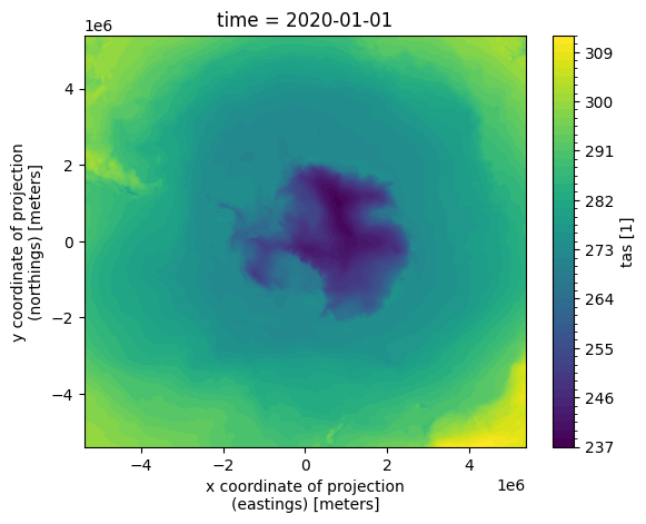
For example, looking at the southern hemisphere sea surface temperature in our example source datastore for the 1st January 2020.
xr.plot.contourf(xr.open_dataset("data/era5/south/tas/2020.nc").isel(time=0).tas, levels=50)
<matplotlib.contour.QuadContourSet at 0x7f175f3bb490>
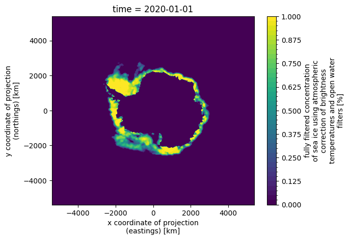
Against the sea ice for the same day is super intuitive to derive from the filesystem naming, by simply changing the respective dataset and variable.
xr.plot.contourf(xr.open_dataset("data/osisaf/south/siconca/2020.nc").isel(time=0).ice_conc, levels=50)
<matplotlib.contour.QuadContourSet at 0x7f16dc022bd0>
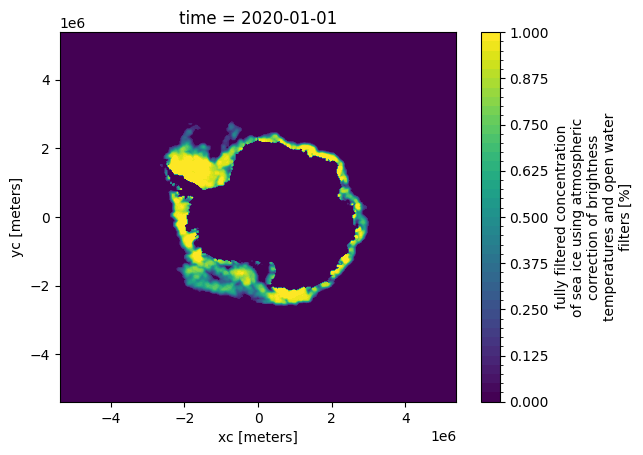
Similarly, switching to the normalised versions (change to /processed/) and/or checking other datasets and/or globbing for datasets that can be opened with xarray.open_mfdataset is equally trivial thanks to this consistency.
xr.plot.contourf(xr.open_dataarray("processed/tutorial_data/osisaf/south/siconca/siconca_abs.nc").isel(time=0), levels=50)
<matplotlib.contour.QuadContourSet at 0x7f16dbf4fb90>
As we’ll see later, extending the library to incorporate additional source data simply adds further entries to the /data directory, with the implementations ultimately following a consistent approach to storing the data to make more complex analysis trivial.
Dask example#
For example, needing to inspect the maximum values for sea surface temperature across all 1990’s and 2000’s data using dask, xarray and glob
from dask.distributed import Client
dfs = glob.glob("data/era5/south/tos/19*.nc") + glob.glob("data/era5/south/tos/20*.nc")
client = Client()
ds = xr.open_mfdataset(dfs, combine="nested", concat_dim="time", parallel=True)
a = ds.groupby("time.year").max("time").max(("yc", "xc"))
m = a.compute()
for y in m.year.values:
print("{} {:.2f}".format(y, float(m.sel(year=y))))
2. Process#
There is a level of consistency (notwithstanding the masks and this currently open issue for clarity) when looking at the processed files. The key here is that the data is normalised as appropriate via the use of processors defined in icenet.data.processors.
The associated normalisation/climatological parameters are then stored in an identified processed data folder, with a corresponding loader.name.json configuration file which takes the form:
!cat loader.tutorial_data.json
{
"sources": {
"era5": {
"name": "tutorial_data",
"implementation": "IceNetERA5PreProcessor",
"anom": [
"zg500",
"zg250"
],
"abs": [
"uas",
"vas"
],
"dates": {
"train": [
"2020_01_01",
"2020_01_02",
"2020_01_03",
"2020_01_04",
"2020_01_05",
"2020_01_06",
"2020_01_07",
"2020_01_08",
"2020_01_09",
"2020_01_10",
"2020_01_11",
"2020_01_12",
"2020_01_13",
"2020_01_14",
"2020_01_15",
"2020_01_16",
"2020_01_17",
"2020_01_18",
"2020_01_19",
"2020_01_20",
"2020_01_21",
"2020_01_22",
"2020_01_23",
"2020_01_24",
"2020_01_25",
"2020_01_26",
"2020_01_27",
"2020_01_28",
"2020_01_29",
"2020_01_30",
"2020_01_31",
"2020_02_01",
"2020_02_02",
"2020_02_03",
"2020_02_04",
"2020_02_05",
"2020_02_06",
"2020_02_07",
"2020_02_08",
"2020_02_09",
"2020_02_10",
"2020_02_11",
"2020_02_12",
"2020_02_13",
"2020_02_14",
"2020_02_15",
"2020_02_16",
"2020_02_17",
"2020_02_18",
"2020_02_19",
"2020_02_20",
"2020_02_21",
"2020_02_22",
"2020_02_23",
"2020_02_24",
"2020_02_25",
"2020_02_26",
"2020_02_27",
"2020_02_28",
"2020_02_29",
"2020_03_01",
"2020_03_02",
"2020_03_03",
"2020_03_04",
"2020_03_05",
"2020_03_06",
"2020_03_07",
"2020_03_08",
"2020_03_09",
"2020_03_10",
"2020_03_11",
"2020_03_12",
"2020_03_13",
"2020_03_14",
"2020_03_15",
"2020_03_16",
"2020_03_17",
"2020_03_18",
"2020_03_19",
"2020_03_20",
"2020_03_21",
"2020_03_22",
"2020_03_23",
"2020_03_24",
"2020_03_25",
"2020_03_26",
"2020_03_27",
"2020_03_28",
"2020_03_29",
"2020_03_30",
"2020_03_31"
],
"val": [
"2020_04_03",
"2020_04_04",
"2020_04_05",
"2020_04_06",
"2020_04_07",
"2020_04_08",
"2020_04_09",
"2020_04_10",
"2020_04_11",
"2020_04_12",
"2020_04_13",
"2020_04_14",
"2020_04_15",
"2020_04_16",
"2020_04_17",
"2020_04_18",
"2020_04_19",
"2020_04_20",
"2020_04_21",
"2020_04_22",
"2020_04_23"
],
"test": [
"2020_04_01",
"2020_04_02"
]
},
"linear_trends": [],
"linear_trend_steps": [
1,
2,
3,
4,
5,
6,
7
],
"meta": [],
"var_files": {
"uas": [
"./processed/tutorial_data/era5/south/uas/uas_abs.nc"
],
"vas": [
"./processed/tutorial_data/era5/south/vas/vas_abs.nc"
],
"zg500": [
"./processed/tutorial_data/era5/south/zg500/zg500_anom.nc"
],
"zg250": [
"./processed/tutorial_data/era5/south/zg250/zg250_anom.nc"
]
}
},
"osisaf": {
"name": "tutorial_data",
"implementation": "IceNetOSIPreProcessor",
"anom": [],
"abs": [
"siconca"
],
"dates": {
"train": [
"2020_01_01",
"2020_01_02",
"2020_01_03",
"2020_01_04",
"2020_01_05",
"2020_01_06",
"2020_01_07",
"2020_01_08",
"2020_01_09",
"2020_01_10",
"2020_01_11",
"2020_01_12",
"2020_01_13",
"2020_01_14",
"2020_01_15",
"2020_01_16",
"2020_01_17",
"2020_01_18",
"2020_01_19",
"2020_01_20",
"2020_01_21",
"2020_01_22",
"2020_01_23",
"2020_01_24",
"2020_01_25",
"2020_01_26",
"2020_01_27",
"2020_01_28",
"2020_01_29",
"2020_01_30",
"2020_01_31",
"2020_02_01",
"2020_02_02",
"2020_02_03",
"2020_02_04",
"2020_02_05",
"2020_02_06",
"2020_02_07",
"2020_02_08",
"2020_02_09",
"2020_02_10",
"2020_02_11",
"2020_02_12",
"2020_02_13",
"2020_02_14",
"2020_02_15",
"2020_02_16",
"2020_02_17",
"2020_02_18",
"2020_02_19",
"2020_02_20",
"2020_02_21",
"2020_02_22",
"2020_02_23",
"2020_02_24",
"2020_02_25",
"2020_02_26",
"2020_02_27",
"2020_02_28",
"2020_02_29",
"2020_03_01",
"2020_03_02",
"2020_03_03",
"2020_03_04",
"2020_03_05",
"2020_03_06",
"2020_03_07",
"2020_03_08",
"2020_03_09",
"2020_03_10",
"2020_03_11",
"2020_03_12",
"2020_03_13",
"2020_03_14",
"2020_03_15",
"2020_03_16",
"2020_03_17",
"2020_03_18",
"2020_03_19",
"2020_03_20",
"2020_03_21",
"2020_03_22",
"2020_03_23",
"2020_03_24",
"2020_03_25",
"2020_03_26",
"2020_03_27",
"2020_03_28",
"2020_03_29",
"2020_03_30",
"2020_03_31"
],
"val": [
"2020_04_01",
"2020_04_02",
"2020_04_03",
"2020_04_04",
"2020_04_05",
"2020_04_06",
"2020_04_07",
"2020_04_08",
"2020_04_09",
"2020_04_10",
"2020_04_11",
"2020_04_12",
"2020_04_13",
"2020_04_14",
"2020_04_15",
"2020_04_16",
"2020_04_17",
"2020_04_18",
"2020_04_19",
"2020_04_20"
],
"test": [
"2020_04_01",
"2020_04_02"
]
},
"linear_trends": [],
"linear_trend_steps": [
1,
2,
3,
4,
5,
6,
7,
8,
9,
10,
11,
12,
13,
14,
15,
16,
17,
18,
19,
20,
21,
22,
23,
24,
25,
26,
27,
28,
29,
30,
31,
32,
33,
34,
35,
36,
37,
38,
39,
40,
41,
42,
43,
44,
45,
46,
47,
48,
49,
50,
51,
52,
53,
54,
55,
56,
57,
58,
59,
60,
61,
62,
63,
64,
65,
66,
67,
68,
69,
70,
71,
72,
73,
74,
75,
76,
77,
78,
79,
80,
81,
82,
83,
84,
85,
86,
87,
88,
89,
90,
91,
92,
93
],
"meta": [],
"var_files": {
"siconca": [
"./processed/tutorial_data/osisaf/south/siconca/siconca_abs.nc"
]
}
},
"meta": {
"name": "tutorial_data",
"implementation": "IceNetMetaPreProcessor",
"anom": [],
"abs": [],
"dates": {
"train": [],
"val": [],
"test": []
},
"linear_trends": [],
"linear_trend_steps": [
1,
2,
3,
4,
5,
6,
7
],
"meta": [
"sin",
"cos",
"land"
],
"var_files": {
"sin": [
"./processed/tutorial_data/meta/south/sin/sin.nc"
],
"cos": [
"./processed/tutorial_data/meta/south/cos/cos.nc"
],
"land": [
"./processed/tutorial_data/meta/south/land/land.nc"
]
}
}
},
"dtype": "float32",
"shape": [
432,
432
],
"missing_dates": []
}
This configuration tracks the various outputs from the normalisation process for each processor used, ensuring that no source data is normalised or modified and can thus be reused across different date ranges easily. At the same time, the caching of this data allows for two additional benefits aside from the obvious separation of preprocessing from data usage. Firstly, the prenormalisation allows uncached datasets to be used directly for predictions and training if desirable and, secondly, it allows multiple datasets to be derived from a single normalisation run which with larger datasets can take a reasonable amount of compute to achieve.
Finally, storing this in a machine and human readable format makes datasets relatively easy to inspect via the loader configuration when you forget what commands you preprocessed with!
Note that the deeper elements of the configuration file aren’t shown for brevity…
Producing preprocessed data videos#
As with data sources, normalised data is easily visualized at the command line by running the icenet_video_data command, where -p specifies path to the directory under /processed/:
!icenet_video_data -p processed/tutorial_data era5,osisaf
[18-02-25 17:31:48 :INFO ] - Looking into processed/tutorial_data
[18-02-25 17:31:48 :INFO ] - Looking at processed/tutorial_data
[18-02-25 17:31:48 :INFO ] - Looking at processed/tutorial_data/era5
[18-02-25 17:31:48 :INFO ] - Looking at processed/tutorial_data/era5/south
[18-02-25 17:31:48 :INFO ] - Looking at processed/tutorial_data/era5/south/normalisation.scale
[18-02-25 17:31:48 :INFO ] - Looking at processed/tutorial_data/era5/south/uas
[18-02-25 17:31:48 :INFO ] - Looking at processed/tutorial_data/era5/south/vas
[18-02-25 17:31:48 :INFO ] - Looking at processed/tutorial_data/era5/south/params
[18-02-25 17:31:48 :INFO ] - Looking at processed/tutorial_data/era5/south/zg500
[18-02-25 17:31:48 :INFO ] - Looking at processed/tutorial_data/era5/south/zg250
[18-02-25 17:31:48 :INFO ] - Looking at processed/tutorial_data/osisaf
[18-02-25 17:31:48 :INFO ] - Looking at processed/tutorial_data/osisaf/south
[18-02-25 17:31:48 :INFO ] - Looking at processed/tutorial_data/osisaf/south/siconca
[18-02-25 17:31:49 :INFO ] - Saving to plot/processed_tutorial_data_osisaf_south_siconca.mp4
[18-02-25 17:31:49 :INFO ] - Saving to plot/processed_tutorial_data_era5_south_zg500.mp4
[18-02-25 17:31:49 :INFO ] - Saving to plot/processed_tutorial_data_era5_south_vas.mp4
[18-02-25 17:31:49 :INFO ] - Saving to plot/processed_tutorial_data_era5_south_uas.mp4
[18-02-25 17:31:49 :INFO ] - Saving to plot/processed_tutorial_data_era5_south_zg250.mp4
[18-02-25 17:31:49 :INFO ] - Inspecting data
[18-02-25 17:31:49 :INFO ] - Inspecting data
[18-02-25 17:31:49 :INFO ] - Inspecting data
[18-02-25 17:31:49 :INFO ] - Inspecting data
[18-02-25 17:31:49 :INFO ] - Inspecting data
[18-02-25 17:31:49 :INFO ] - Initialising plot
[18-02-25 17:31:50 :INFO ] - Initialising plot
[18-02-25 17:31:50 :INFO ] - Initialising plot
[18-02-25 17:31:50 :INFO ] - Initialising plot
[18-02-25 17:31:50 :INFO ] - Initialising plot
[18-02-25 17:31:51 :INFO ] - Animating
[18-02-25 17:31:51 :INFO ] - Animating
[18-02-25 17:31:51 :INFO ] - Animating
[18-02-25 17:31:51 :INFO ] - Animating
[18-02-25 17:31:51 :INFO ] - Saving plot to plot/processed_tutorial_data_osisaf_south_siconca.mp4
[18-02-25 17:31:51 :INFO ] - Animating
[18-02-25 17:31:52 :INFO ] - Saving plot to plot/processed_tutorial_data_era5_south_zg500.mp4
[18-02-25 17:31:52 :INFO ] - Saving plot to plot/processed_tutorial_data_era5_south_uas.mp4
[18-02-25 17:31:52 :INFO ] - Saving plot to plot/processed_tutorial_data_era5_south_vas.mp4
[18-02-25 17:31:52 :INFO ] - Saving plot to plot/processed_tutorial_data_era5_south_zg250.mp4
[18-02-25 17:32:49 :INFO ] - Produced plot/processed_tutorial_data_osisaf_south_siconca.mp4
[18-02-25 17:40:54 :INFO ] - Produced plot/processed_tutorial_data_era5_south_zg250.mp4
[18-02-25 17:41:00 :INFO ] - Produced plot/processed_tutorial_data_era5_south_zg500.mp4
[18-02-25 17:41:07 :INFO ] - Produced plot/processed_tutorial_data_era5_south_uas.mp4
[18-02-25 17:41:09 :INFO ] - Produced plot/processed_tutorial_data_era5_south_vas.mp4
from IPython.display import Video
Video("plot/processed_tutorial_data_era5_south_uas.mp4", embed=True, width=800)
3. Train#
Training outputs are stored in their respectively named folders using the name provided from the commands icenet_train or run_train_ensemble respectively. The contents of these folders differ slightly, based simply on the number of runs executed.
os.listdir("results/networks")
['tutorial_testrun']
The output from the single run provides two appropriately named files, the JSON of the history object from the run and the weights of the network after training.
glob.glob("results/networks/tutorial_testrun/**", recursive=True)
['results/networks/tutorial_testrun/',
'results/networks/tutorial_testrun/tutorial_testrun.network_tutorial_data.42.h5',
'results/networks/tutorial_testrun/tutorial_testrun.model_tutorial_data.42',
'results/networks/tutorial_testrun/tutorial_testrun.model_tutorial_data.42/variables',
'results/networks/tutorial_testrun/tutorial_testrun.model_tutorial_data.42/variables/variables.data-00000-of-00001',
'results/networks/tutorial_testrun/tutorial_testrun.model_tutorial_data.42/variables/variables.index',
'results/networks/tutorial_testrun/tutorial_testrun.model_tutorial_data.42/assets',
'results/networks/tutorial_testrun/tutorial_testrun.model_tutorial_data.42/saved_model.pb',
'results/networks/tutorial_testrun/tutorial_testrun.model_tutorial_data.42/fingerprint.pb',
'results/networks/tutorial_testrun/tutorial_testrun.model_tutorial_data.42/keras_metadata.pb',
'results/networks/tutorial_testrun/tutorial_testrun_42_history.json',
'results/networks/tutorial_testrun/tutorial_testrun.model_tutorial_data.42.results.json']
Similarly, the ensemble outputs the same files across each individual run, distinguished by the seed (Generated using the second notebook).
Note This was generated via the second notebook using the icenet-pipeline, and so is in the ../notebook-pipeline directory.
glob.glob("../notebook-pipeline/results/networks/tutorial_south_ensemble/**/*.h5", recursive=True) + glob.glob("../notebook-pipeline/results/networks/tutorial_south_ensemble/**/*.json", recursive=True)
['../notebook-pipeline/results/networks/tutorial_south_ensemble/tutorial_south_ensemble.network_tutorial_pipeline_south.42.h5',
'../notebook-pipeline/results/networks/tutorial_south_ensemble/tutorial_south_ensemble.network_tutorial_pipeline_south.46.h5',
'../notebook-pipeline/results/networks/tutorial_south_ensemble/tutorial_south_ensemble_46_history.json',
'../notebook-pipeline/results/networks/tutorial_south_ensemble/tutorial_south_ensemble_42_history.json',
'../notebook-pipeline/results/networks/tutorial_south_ensemble/tutorial_south_ensemble.model_tutorial_pipeline_south.46.results.json',
'../notebook-pipeline/results/networks/tutorial_south_ensemble/tutorial_south_ensemble.model_tutorial_pipeline_south.42.results.json']
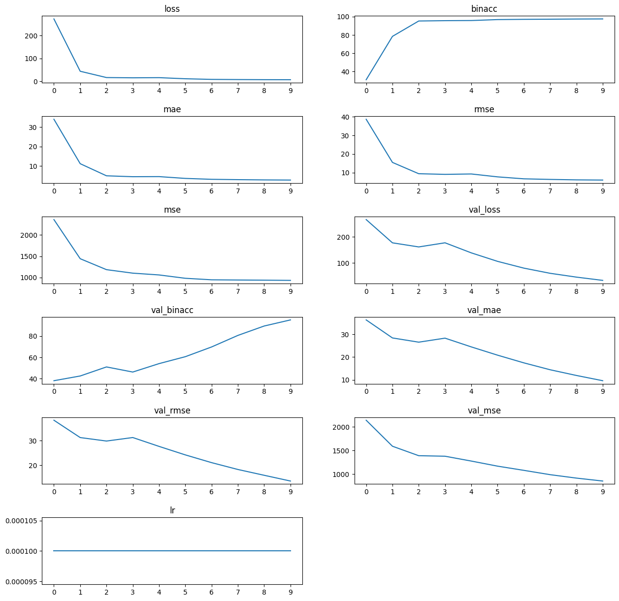
with open("../notebook-pipeline/results/networks/tutorial_south_ensemble/tutorial_south_ensemble_42_history.json") as fh:
history = json.load(fh)
# Quick and dirty visualisation
fig = plt.figure(figsize=(int(len(history.keys())/2) * 3, 15))
fig.tight_layout()
plt.subplots_adjust(hspace=0.5)
for i, k in enumerate(history.keys()):
ax = fig.add_subplot(int(len(history.keys())/2) + len(history.keys())%2, 2, i+1)
ax.plot(history[k].keys(), history[k].values())
ax.set_title(k)
fig.show()
/tmp/ipykernel_15022/727979000.py:15: UserWarning: FigureCanvasAgg is non-interactive, and thus cannot be shown
fig.show()
It’s important to note that other outputs result, depending on arguments provided and configuration, from icenet_train and run_icenet_ensemble. Both tensorboard and WandB outputs can be provided and, in the case of the latter, automatically uploaded when using the CLI tools. The output files are also retained in the run folders, with the latter ensemble members being stored in the /ensemble/<ensembleName>/<ensembleName>-<runNumber> directory:
os.listdir("../notebook-pipeline/ensemble/tutorial_south_ensemble/tutorial_south_ensemble-0")
['bashpc.sh',
'icenet_predict.sh.j2',
'jasmin.sh',
'local.sh',
'icenet_train.sh',
'train.6288960.node022.42.out',
'train.6288960.node022.42.err',
'data',
'ENVS',
'ENVS.example',
'loader.tutorial_pipeline_south.json',
'dataset_config.tutorial_pipeline_south.json',
'network_datasets',
'processed',
'results',
'logs']
Depending on the mechanism (in this case SLURM on our HPC) used to run the ensemble, the log files provide the full output from the run:
!cat ../notebook-pipeline/ensemble/tutorial_south_ensemble/tutorial_south_ensemble-0/train.*.node*.42.out
START 2025-02-18 15:44:47
Running icenet_train -v tutorial_pipeline_south tutorial_south_ensemble 42 -b 4 -e 10 -m -qs 4 -w 4 -s default -n 0.6
Model: "model"
__________________________________________________________________________________________________
Layer (type) Output Shape Param # Connected to
==================================================================================================
input_1 (InputLayer) [(None, 432, 432, 15)] 0 []
conv2d (Conv2D) (None, 432, 432, 38) 5168 ['input_1[0][0]']
conv2d_1 (Conv2D) (None, 432, 432, 38) 13034 ['conv2d[0][0]']
batch_normalization (Batch (None, 432, 432, 38) 152 ['conv2d_1[0][0]']
Normalization)
max_pooling2d (MaxPooling2 (None, 216, 216, 38) 0 ['batch_normalization[0][0]']
D)
conv2d_2 (Conv2D) (None, 216, 216, 76) 26068 ['max_pooling2d[0][0]']
conv2d_3 (Conv2D) (None, 216, 216, 76) 52060 ['conv2d_2[0][0]']
batch_normalization_1 (Bat (None, 216, 216, 76) 304 ['conv2d_3[0][0]']
chNormalization)
max_pooling2d_1 (MaxPoolin (None, 108, 108, 76) 0 ['batch_normalization_1[0][0]'
g2D) ]
conv2d_4 (Conv2D) (None, 108, 108, 152) 104120 ['max_pooling2d_1[0][0]']
conv2d_5 (Conv2D) (None, 108, 108, 152) 208088 ['conv2d_4[0][0]']
batch_normalization_2 (Bat (None, 108, 108, 152) 608 ['conv2d_5[0][0]']
chNormalization)
max_pooling2d_2 (MaxPoolin (None, 54, 54, 152) 0 ['batch_normalization_2[0][0]'
g2D) ]
conv2d_6 (Conv2D) (None, 54, 54, 152) 208088 ['max_pooling2d_2[0][0]']
conv2d_7 (Conv2D) (None, 54, 54, 152) 208088 ['conv2d_6[0][0]']
batch_normalization_3 (Bat (None, 54, 54, 152) 608 ['conv2d_7[0][0]']
chNormalization)
max_pooling2d_3 (MaxPoolin (None, 27, 27, 152) 0 ['batch_normalization_3[0][0]'
g2D) ]
conv2d_8 (Conv2D) (None, 27, 27, 304) 416176 ['max_pooling2d_3[0][0]']
conv2d_9 (Conv2D) (None, 27, 27, 304) 832048 ['conv2d_8[0][0]']
batch_normalization_4 (Bat (None, 27, 27, 304) 1216 ['conv2d_9[0][0]']
chNormalization)
up_sampling2d (UpSampling2 (None, 54, 54, 304) 0 ['batch_normalization_4[0][0]'
D) ]
conv2d_10 (Conv2D) (None, 54, 54, 152) 184984 ['up_sampling2d[0][0]']
concatenate (Concatenate) (None, 54, 54, 304) 0 ['batch_normalization_3[0][0]'
, 'conv2d_10[0][0]']
conv2d_11 (Conv2D) (None, 54, 54, 152) 416024 ['concatenate[0][0]']
conv2d_12 (Conv2D) (None, 54, 54, 152) 208088 ['conv2d_11[0][0]']
batch_normalization_5 (Bat (None, 54, 54, 152) 608 ['conv2d_12[0][0]']
chNormalization)
up_sampling2d_1 (UpSamplin (None, 108, 108, 152) 0 ['batch_normalization_5[0][0]'
g2D) ]
conv2d_13 (Conv2D) (None, 108, 108, 152) 92568 ['up_sampling2d_1[0][0]']
concatenate_1 (Concatenate (None, 108, 108, 304) 0 ['batch_normalization_2[0][0]'
) , 'conv2d_13[0][0]']
conv2d_14 (Conv2D) (None, 108, 108, 152) 416024 ['concatenate_1[0][0]']
conv2d_15 (Conv2D) (None, 108, 108, 152) 208088 ['conv2d_14[0][0]']
batch_normalization_6 (Bat (None, 108, 108, 152) 608 ['conv2d_15[0][0]']
chNormalization)
up_sampling2d_2 (UpSamplin (None, 216, 216, 152) 0 ['batch_normalization_6[0][0]'
g2D) ]
conv2d_16 (Conv2D) (None, 216, 216, 76) 46284 ['up_sampling2d_2[0][0]']
concatenate_2 (Concatenate (None, 216, 216, 152) 0 ['batch_normalization_1[0][0]'
) , 'conv2d_16[0][0]']
conv2d_17 (Conv2D) (None, 216, 216, 76) 104044 ['concatenate_2[0][0]']
conv2d_18 (Conv2D) (None, 216, 216, 76) 52060 ['conv2d_17[0][0]']
batch_normalization_7 (Bat (None, 216, 216, 76) 304 ['conv2d_18[0][0]']
chNormalization)
up_sampling2d_3 (UpSamplin (None, 432, 432, 76) 0 ['batch_normalization_7[0][0]'
g2D) ]
conv2d_19 (Conv2D) (None, 432, 432, 38) 11590 ['up_sampling2d_3[0][0]']
concatenate_3 (Concatenate (None, 432, 432, 76) 0 ['conv2d_1[0][0]',
) 'conv2d_19[0][0]']
conv2d_20 (Conv2D) (None, 432, 432, 38) 26030 ['concatenate_3[0][0]']
conv2d_21 (Conv2D) (None, 432, 432, 38) 13034 ['conv2d_20[0][0]']
conv2d_22 (Conv2D) (None, 432, 432, 38) 13034 ['conv2d_21[0][0]']
conv2d_23 (Conv2D) (None, 432, 432, 7) 273 ['conv2d_22[0][0]']
==================================================================================================
Total params: 3869471 (14.76 MB)
Trainable params: 3867267 (14.75 MB)
Non-trainable params: 2204 (8.61 KB)
__________________________________________________________________________________________________
Epoch 1/10
23/Unknown - 26s 312ms/step - loss: 272.4839 - binacc: 30.9099 - mae: 34.0224 - rmse: 38.7146 - mse: 2362.2986
Epoch 1: val_rmse improved from inf to 38.31770, saving model to ./results/networks/tutorial_south_ensemble/tutorial_south_ensemble.network_tutorial_pipeline_south.42.h5
23/23 [==============================] - 29s 461ms/step - loss: 272.4839 - binacc: 30.9099 - mae: 34.0224 - rmse: 38.7146 - mse: 2362.2986 - val_loss: 266.9253 - val_binacc: 38.0610 - val_mae: 36.2745 - val_rmse: 38.3177 - val_mse: 2141.5354 - lr: 1.0000e-04
Epoch 2/10
23/23 [==============================] - ETA: 0s - loss: 43.5792 - binacc: 78.4264 - mae: 11.1747 - rmse: 15.4826 - mse: 1440.9474
Epoch 2: val_rmse improved from 38.31770 to 31.25504, saving model to ./results/networks/tutorial_south_ensemble/tutorial_south_ensemble.network_tutorial_pipeline_south.42.h5
23/23 [==============================] - 4s 191ms/step - loss: 43.5792 - binacc: 78.4264 - mae: 11.1747 - rmse: 15.4826 - mse: 1440.9474 - val_loss: 177.5951 - val_binacc: 42.5011 - val_mae: 28.3588 - val_rmse: 31.2550 - val_mse: 1591.5531 - lr: 1.0000e-04
Epoch 3/10
23/23 [==============================] - ETA: 0s - loss: 16.0391 - binacc: 95.2752 - mae: 4.9435 - rmse: 9.3928 - mse: 1183.3113
Epoch 3: val_rmse improved from 31.25504 to 29.83513, saving model to ./results/networks/tutorial_south_ensemble/tutorial_south_ensemble.network_tutorial_pipeline_south.42.h5
23/23 [==============================] - 4s 191ms/step - loss: 16.0391 - binacc: 95.2752 - mae: 4.9435 - rmse: 9.3928 - mse: 1183.3113 - val_loss: 161.8254 - val_binacc: 51.0065 - val_mae: 26.5028 - val_rmse: 29.8351 - val_mse: 1391.3385 - lr: 1.0000e-04
Epoch 4/10
23/23 [==============================] - ETA: 0s - loss: 14.9025 - binacc: 95.6252 - mae: 4.4781 - rmse: 9.0539 - mse: 1101.0161
Epoch 4: val_rmse did not improve from 29.83513
23/23 [==============================] - 4s 192ms/step - loss: 14.9025 - binacc: 95.6252 - mae: 4.4781 - rmse: 9.0539 - mse: 1101.0161 - val_loss: 177.7188 - val_binacc: 46.2075 - val_mae: 28.2660 - val_rmse: 31.2659 - val_mse: 1380.2626 - lr: 1.0000e-04
Epoch 5/10
23/23 [==============================] - ETA: 0s - loss: 15.5931 - binacc: 95.7887 - mae: 4.5274 - rmse: 9.2613 - mse: 1058.7959
Epoch 5: val_rmse improved from 29.83513 to 27.65393, saving model to ./results/networks/tutorial_south_ensemble/tutorial_south_ensemble.network_tutorial_pipeline_south.42.h5
23/23 [==============================] - 5s 196ms/step - loss: 15.5931 - binacc: 95.7887 - mae: 4.5274 - rmse: 9.2613 - mse: 1058.7959 - val_loss: 139.0287 - val_binacc: 54.1188 - val_mae: 24.4239 - val_rmse: 27.6539 - val_mse: 1277.8448 - lr: 1.0000e-04
Epoch 6/10
23/23 [==============================] - ETA: 0s - loss: 10.7766 - binacc: 96.8123 - mae: 3.6016 - rmse: 7.6992 - mse: 980.0773
Epoch 6: val_rmse improved from 27.65393 to 24.18846, saving model to ./results/networks/tutorial_south_ensemble/tutorial_south_ensemble.network_tutorial_pipeline_south.42.h5
23/23 [==============================] - 5s 198ms/step - loss: 10.7766 - binacc: 96.8123 - mae: 3.6016 - rmse: 7.6992 - mse: 980.0773 - val_loss: 106.3671 - val_binacc: 60.6351 - val_mae: 20.7960 - val_rmse: 24.1885 - val_mse: 1170.1218 - lr: 1.0000e-04
Epoch 7/10
23/23 [==============================] - ETA: 0s - loss: 8.0344 - binacc: 97.0929 - mae: 3.1395 - rmse: 6.6478 - mse: 944.3714
Epoch 7: val_rmse improved from 24.18846 to 21.02781, saving model to ./results/networks/tutorial_south_ensemble/tutorial_south_ensemble.network_tutorial_pipeline_south.42.h5
23/23 [==============================] - 5s 193ms/step - loss: 8.0344 - binacc: 97.0929 - mae: 3.1395 - rmse: 6.6478 - mse: 944.3714 - val_loss: 80.3857 - val_binacc: 69.7870 - val_mae: 17.4203 - val_rmse: 21.0278 - val_mse: 1081.2783 - lr: 1.0000e-04
Epoch 8/10
23/23 [==============================] - ETA: 0s - loss: 7.2828 - binacc: 97.2400 - mae: 2.9632 - rmse: 6.3293 - mse: 939.5836
Epoch 8: val_rmse improved from 21.02781 to 18.24148, saving model to ./results/networks/tutorial_south_ensemble/tutorial_south_ensemble.network_tutorial_pipeline_south.42.h5
23/23 [==============================] - 5s 201ms/step - loss: 7.2828 - binacc: 97.2400 - mae: 2.9632 - rmse: 6.3293 - mse: 939.5836 - val_loss: 60.4938 - val_binacc: 80.6337 - val_mae: 14.3917 - val_rmse: 18.2415 - val_mse: 989.9238 - lr: 1.0000e-04
Epoch 9/10
23/23 [==============================] - ETA: 0s - loss: 6.7340 - binacc: 97.4289 - mae: 2.8347 - rmse: 6.0861 - mse: 935.8147
Epoch 9: val_rmse improved from 18.24148 to 15.87550, saving model to ./results/networks/tutorial_south_ensemble/tutorial_south_ensemble.network_tutorial_pipeline_south.42.h5
23/23 [==============================] - 5s 196ms/step - loss: 6.7340 - binacc: 97.4289 - mae: 2.8347 - rmse: 6.0861 - mse: 935.8147 - val_loss: 45.8190 - val_binacc: 89.4631 - val_mae: 11.8855 - val_rmse: 15.8755 - val_mse: 917.3613 - lr: 1.0000e-04
Epoch 10/10
23/23 [==============================] - ETA: 0s - loss: 6.5082 - binacc: 97.5380 - mae: 2.7562 - rmse: 5.9832 - mse: 930.7341
Epoch 10: val_rmse improved from 15.87550 to 13.53251, saving model to ./results/networks/tutorial_south_ensemble/tutorial_south_ensemble.network_tutorial_pipeline_south.42.h5
23/23 [==============================] - 5s 195ms/step - loss: 6.5082 - binacc: 97.5380 - mae: 2.7562 - rmse: 5.9832 - mse: 930.7341 - val_loss: 33.2926 - val_binacc: 95.1965 - val_mae: 9.5865 - val_rmse: 13.5325 - val_mse: 855.3213 - lr: 1.0000e-04
FINISH 2025-02-18 15:46:38
Of course in the case of individual runs using icenet_train this output will have been presented to stdout/stderr (the screen) whilst running…
4. Predict#
The training runs provide insight into the training of the network (using the CLI in a very simple fashion) but the predictions produce actual forecast output to be studied or utilised. This can be evaluated as befits the user in comparison to the original SIC data or any other source to validate the forecasts. Obviously with our notebook network these won’t be accurate but in real use you’d be expecting to produce comparable forecasts with the physics based data used to train the network.
All outputs for prediction runs using either icenet_predict or run_predict_ensemble are stored in results/predict. For our notebook test and ensemble runs we can see the folder structure is similar to the training outputs, with folders named using the identifier:
glob.glob("../notebook-pipeline/results/predict/**")
['../notebook-pipeline/results/predict/tutorial_south_ensemble_forecast',
'../notebook-pipeline/results/predict/tutorial_south_ensemble_forecast.nc']
os.listdir("../notebook-pipeline/results/predict/tutorial_south_ensemble_forecast")
['tutorial_south_ensemble.46', 'tutorial_south_ensemble.42']
os.listdir("../notebook-pipeline/results/predict/tutorial_south_ensemble_forecast/tutorial_south_ensemble.42")
['2020_04_01.npy', '2020_04_02.npy']
The prediction per-network folder contains output from the network for the inputs provided, with the dates being the forecast start date. These files correspond to the original dates we provided in the first notebook.
!cat testdates.csv
2020-04-01
2020-04-02
In the loader are also contained outputs and weights. The former “outputs” are the generated outputs for the network that would’ve been used for training. Remember, that to produce a forecast we use an input linear trend SIC channel set, alongside the atmospheric and other data channels. The weights is the collection of sample weights associated to the input set. These are really provided for debugging purposes, but may also be of some analytical interest in some cases.
With the run of icenet_output as shown in the first notebook, these numpy-saved outputs are converted to a CF-compliant NetCDF that can be forwarded on or usefully analysed.
Plotting a forecast#
The following snippet uses one of these NetCDF’s for plotting a forecast:
from icenet.plotting.video import xarray_to_video as xvid
from icenet.data.sic.mask import Masks
ds = xr.open_dataset("../notebook-pipeline/results/predict/tutorial_south_ensemble_forecast.nc")
land_mask = Masks(south=True, north=False).get_land_mask()
ds.info()
xarray.Dataset {
dimensions:
time = 2 ;
yc = 432 ;
xc = 432 ;
leadtime = 7 ;
variables:
int32 Lambert_Azimuthal_Grid() ;
Lambert_Azimuthal_Grid:grid_mapping_name = lambert_azimuthal_equal_area ;
Lambert_Azimuthal_Grid:longitude_of_projection_origin = 0.0 ;
Lambert_Azimuthal_Grid:latitude_of_projection_origin = -90.0 ;
Lambert_Azimuthal_Grid:false_easting = 0.0 ;
Lambert_Azimuthal_Grid:false_northing = 0.0 ;
Lambert_Azimuthal_Grid:semi_major_axis = 6378137.0 ;
Lambert_Azimuthal_Grid:inverse_flattening = 298.257223563 ;
Lambert_Azimuthal_Grid:proj4_string = +proj=laea +lon_0=0 +datum=WGS84 +ellps=WGS84 +lat_0=-90.0 ;
float32 sic_mean(time, yc, xc, leadtime) ;
sic_mean:long_name = mean sea ice area fraction across ensemble runs of icenet model ;
sic_mean:standard_name = sea_ice_area_fraction ;
sic_mean:short_name = sic ;
sic_mean:valid_min = 0 ;
sic_mean:valid_max = 1 ;
sic_mean:ancillary_variables = sic_stddev ;
sic_mean:grid_mapping = Lambert_Azimuthal_Grid ;
sic_mean:units = 1 ;
float32 sic_stddev(time, yc, xc, leadtime) ;
sic_stddev:long_name = total uncertainty (one standard deviation) of concentration of sea ice ;
sic_stddev:standard_name = sea_ice_area_fraction standard_error ;
sic_stddev:valid_min = 0 ;
sic_stddev:valid_max = 1 ;
sic_stddev:grid_mapping = Lambert_Azimuthal_Grid ;
sic_stddev:units = 1 ;
int64 ensemble_members(time) ;
ensemble_members:long_name = number of ensemble members used to create this prediction ;
ensemble_members:short_name = ensemble_members ;
datetime64[ns] time(time) ;
time:long_name = reference time of product ;
time:standard_name = time ;
time:axis = T ;
int64 leadtime(leadtime) ;
leadtime:long_name = leadtime of forecast in relation to reference time ;
leadtime:short_name = leadtime ;
datetime64[ns] forecast_date(time, leadtime) ;
float64 xc(xc) ;
xc:long_name = x coordinate of projection (eastings) ;
xc:standard_name = projection_x_coordinate ;
xc:units = 1000 meter ;
xc:axis = X ;
float64 yc(yc) ;
yc:long_name = y coordinate of projection (northings) ;
yc:standard_name = projection_y_coordinate ;
yc:units = 1000 meter ;
yc:axis = Y ;
float32 lat(yc, xc) ;
lat:long_name = latitude coordinate ;
lat:standard_name = latitude ;
lat:units = arc_degree ;
float32 lon(yc, xc) ;
lon:long_name = longitude coordinate ;
lon:standard_name = longitude ;
lon:units = arc_degree ;
// global attributes:
:Conventions = CF-1.6 ACDD-1.3 ;
:comments = ;
:creator_email = jambyr@bas.ac.uk ;
:creator_institution = British Antarctic Survey ;
:creator_name = James Byrne ;
:creator_url = www.bas.ac.uk ;
:date_created = 2025-02-18 ;
:geospatial_bounds_crs = EPSG:6932 ;
:geospatial_lat_min = -90.0 ;
:geospatial_lat_max = -16.62393 ;
:geospatial_lon_min = -180.0 ;
:geospatial_lon_max = 180.0 ;
:geospatial_vertical_min = 0.0 ;
:geospatial_vertical_max = 0.0 ;
:history = 2025-02-18 15:53:31.886924 - creation ;
:id = IceNet 0.2.9_dev ;
:institution = British Antarctic Survey ;
:keywords = 'Earth Science > Cryosphere > Sea Ice > Sea Ice Concentration
Earth Science > Oceans > Sea Ice > Sea Ice Concentration
Earth Science > Climate Indicators > Cryospheric Indicators > Sea Ice
Geographic Region > Southern Hemisphere ;
:keywords_vocabulary = GCMD Science Keywords ;
:license = Open Government Licece (OGL) V3 ;
:naming_authority = uk.ac.bas ;
:platform = BAS HPC ;
:product_version = 0.2.9_dev ;
:project = IceNet ;
:publisher_email = ;
:publisher_institution = British Antarctic Survey ;
:publisher_url = ;
:source =
IceNet model generation at v0.2.9_dev
;
:spatial_resolution = 25.0 km grid spacing ;
:standard_name_vocabulary = CF Standard Name Table v27 ;
:summary =
This is an output of sea ice concentration predictions from the
IceNet run in an ensemble, with postprocessing to determine
the mean and standard deviation across the runs.
;
:time_coverage_start = 2020-04-02T00:00:00 ;
:time_coverage_end = 2020-04-09T00:00:00 ;
:time_coverage_duration = P1D ;
:time_coverage_resolution = P1D ;
:title = Sea Ice Concentration Prediction ;
}
forecast_date = ds.time.values[0]
print(forecast_date)
2020-04-01T00:00:00.000000000
fc = ds.sic_mean.isel(time=0).drop_vars("time").rename(dict(leadtime="time"))
fc['time'] = [pd.to_datetime(forecast_date) \
+ dt.timedelta(days=int(e)) for e in fc.time.values]
anim = xvid(fc, 15, figsize=(4, 4), mask=land_mask, north=False, south=True)
HTML(anim.to_jshtml())
Obviously, with the size and training of the notebook dataset this is not a particularly useful forecast but the ease of generating a visual is hopefully apparent. Also, this segways nicely into the next notebook as we’ve started to introduce leverages methods and classes directly from the icenet API itself.
Summary#
In this notebook we’ve explored the data assets that are stored based on the end to end run of the pipeline, hopefully enough to make the user aware of the structuring of the run directory when using either single-run or ensemble-based mechanisms of execution. Using illustrative but minimal data, we’ve highlighted the potential use of these assets to generate visual products and give insight into the processing that takes place.
Those interested in running forecasts with a properly scaled training and prediction set of data should now be able to consider doing so using the CLI commands. However, the CLI commands only expose an illustrative set of commands at present, whereas leveraging the API directly affords far more flexibility. This is explored in the remaining notebooks:
Library usage
04.library_usage.ipynb: understand how to programmatically perform an end to end run.
Version#
IceNet Codebase: v0.2.9